Find the detailed code and more about bootstrap in my github
Introduction to Bootstrap
Bootstrap is a powerful tool widely used by statisticians and data scientists to quantify the uncertainty associated with estimated parameters in the context of statistical learning methods. If we want to account for the uncertainty of the parameters in a model, bootstrapping can help. Instead of using the complete data to estimate them once, we can repeat the process many times on the different samples generated with replacement to obtain a vector of estimates. Then, it becomes possible to estimate some statistical properties of the parameters, such as its standard-deviation and confidence intervals. For instance, in linear regression, we can use bootstrap to estimate the variance of the coefficients (betas) and consequently understand how reliable are they. However, it would not make any sense to repeat such tasks with the same dataset, as the parameters would always return the equal, and the variance would be zero. Instead, bootstrap consists of creating new resampled datasets. Some machine learning methods have already incorporated bootstrap into its algorithm, more notably Random Forests, that use bagging (bootstrap aggregating) to reduce the complexity of models that overfit the training data. In this work, we will explore bootstrap with Regression models. We will be doing a regression with a dataset from the year from 2015 with GDP-Per-Capita and life expectancy from most countries in the world. We want to model the relationship between these two variables. In the context of bootstrap, the first step would be to create the mentioned resampled datasets, as we can see in figure 1.
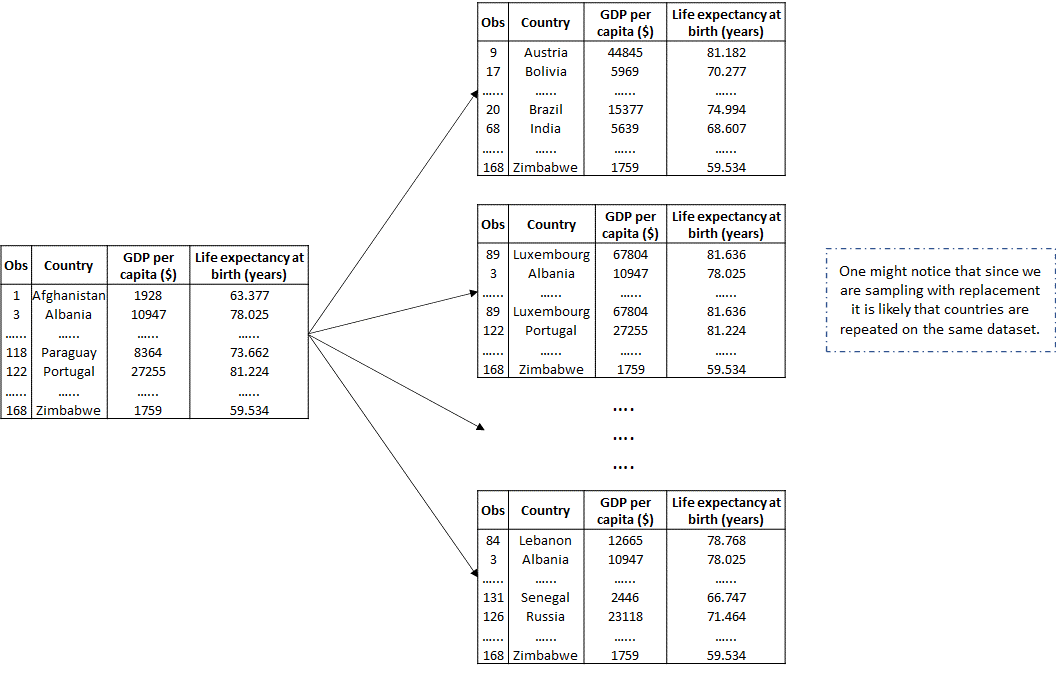
FIGURE 1. A graphical illustration of the bootstrap approach on a dataset containing n = 168 observations. Each bootstrap data set contains n observations, sampled with replacement from the original data set. Each bootstrap data set is used to obtain one estimate of the parameters which will compose the final vector/distribution.
Bootstrap to quantify Uncertainty
When it comes to machine learning, the conclusions that can be drawn from a model are as important as they’re reliability. To ensure that a model is reliable it must not only achieve a good accuracy but it must also be constant on its results. If we train the model $n$ different times with samples that were drawn from the same dataset, we expect the mode to yield similar results every time, otherwise it might indicate that the model will work in some cases but not in others.
Concerning a regression model, we can calculate the parameters of the betas and intercept such as the mean and standard deviation. A high standard deviation will indicate a problem in the confidence of the model. In the ideal cenario, the parameters will show a normal distribution.
Algorithm
The logic of bootstrap is quite simple and can be captured in simple lines of code, or pseudocode. In the end, it comes down to repeatedly perform a task with random samples (with replacement). 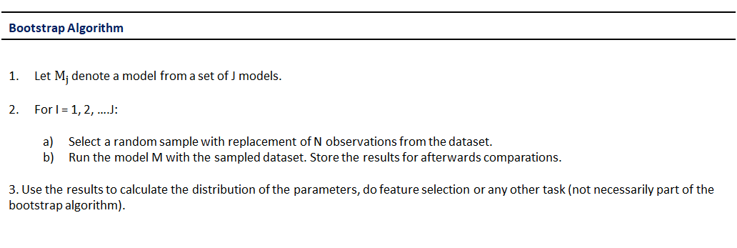
FIGURE 3. The Bootstrap algorithm
Bootstrap in a Polynomial Regression
Does the richness of a country imply in a more lasting life expectancy? Easy question, the answer is Yes. At least in most cases. We will be working with a dataset from the World Bank to try to model the relationship of these variables.
The variables are the following:
GDP-Per-Capital:The total amount of richness per person in a country.The life expectancy:The number of years expected for someone to live in a country.
Lets have a first look in the data with a scatter plot.
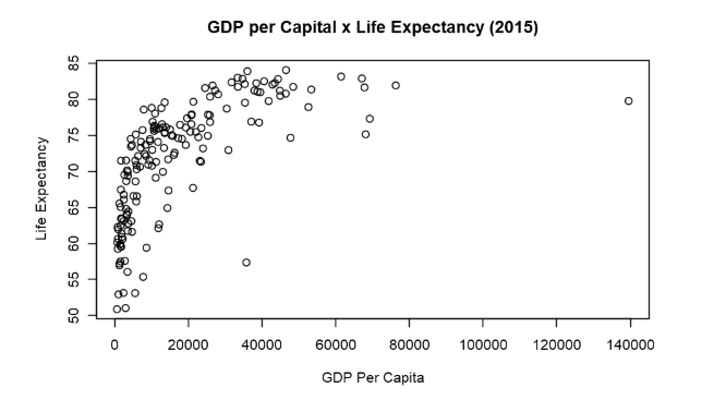
FIGURE 4. GDP per Capita x Life Expectancy
There is a clear relationship in the data. Countries with higher GDP-Per-Capita have an also higher life expectancy. The reason is not hard to guess. Better infrastructure, better health systems, sanitation education and all that comes with economic development. It is worth noticing that we are working with GPD-per-Capita instead of GDP. The difference is that the number is divided by the number of citizens so that the number is not biased towards countries that have a vast population (such as China and India). However, it is also clear that the relationship between these variables is not linear, and therefore cannot be modelled by linear regression. Instead, we will use polynomial regression.
In the next steps we will have a look in the data and create a regression of second degree.
data <- read.csv('life-expectancy-vs-gdp-per-capita.csv') # import the data
colnames(data) <- c('Entity', 'code', 'Year', 'l_expect', 'GDP_per_capita', 'Pop') # improve names
data <- na.omit(data) # remove NA's
head(data)
| Id | Entity | code | Year | l_expect | GDP_per_capita | Pop |
|---|---|---|---|---|---|---|
| 1 | Afghanistan | AFG | 2015 | 63.377 | 1928 | 34414000 |
| 3 | Albania | ALB | 2015 | 78.025 | 10947 | 2891000 |
| 4 | Algeria | DZA | 2015 | 76.090 | 13024 | 39728000 |
| 8 | Angola | AGO | 2015 | 59.398 | 8631 | 27884000 |
| 11 | Argentina | ARG | 2015 | 76.068 | 19316 | 43075000 |
Next step, make the polynomial regression:
model <- lm(data$l_expect ~ data$GDP_per_capita + I(data$GDP_per_capita^2))
summary(model)
Call:
lm(formula = data$l_expect ~ data$GDP_per_capita + I(data$GDP_per_capita^2))

Residuals:
     Min       1Q   Median       3Q      Max
-23.3124  -2.1618   0.6404   3.1210   9.8065

Coefficients:
                           Estimate Std. Error t value Pr(>|t|)
(Intercept)               6.155e+01  8.096e-01   76.02  < 2e-16 ***
data$GDP_per_capita       1.021e-03  9.952e-05   10.26  < 2e-16 ***
I(data$GDP_per_capita^2) -1.359e-08  2.148e-09   -6.33 2.42e-09 ***
---
Signif. codes:  0 '***' 0.001 '**' 0.01 '*' 0.05 '.' 0.1 ' ' 1

Residual standard error: 5.048 on 158 degrees of freedom
Multiple R-squared:  0.6137,Adjusted R-squared:  0.6088
F-statistic: 125.5 on 2 and 158 DF,  p-value: < 2.2e-16
Our regressions seem to have a good fit. Our parameters have statistical significance, and we have found a satisfactory adjusted R-squared. Let’s plot the line in the dataset.
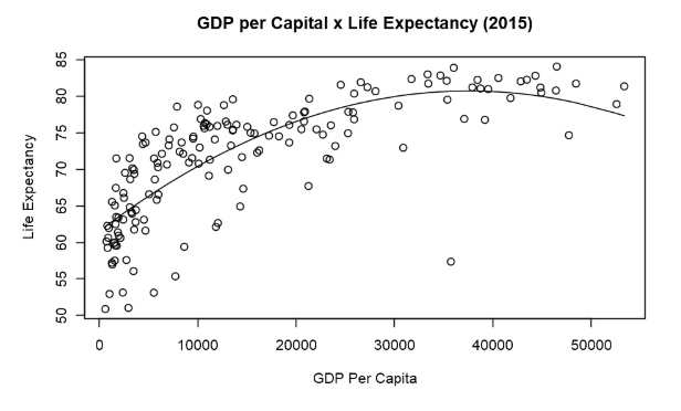
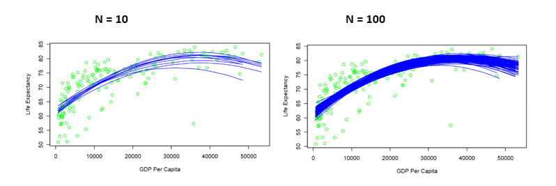
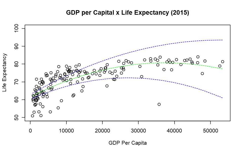
When making a prediction, we do not want to be limited to the point of our model. We want to find a confidence interval. We will find the confidence interval creating bootstrapped models. First let’s make a plot with n models, where n equals 10 and 100.
Model Parameters
Making use of every model above we have found or model parameters and their statistical distribution. Lets plot the data of every beta and intercept.
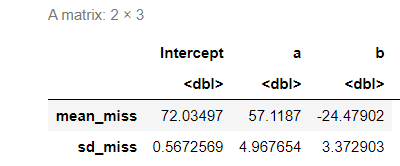
The Distribution of the Betas
 FIGURE 2. A graphical illustration of the distribution of the parameters of a polynomial regression of second degree and the number of repetitions (n = 1000). The parameters follow a gaussian distribution.
Now lets plot the regression with upper and lower lines - a condidence interval of 95%.
Bootstraped Model with Confidenc e Interval
That’s all for now, thanks for reading!
